pygmt.Figure.fill_between
- Figure.fill_between(x, y, y2=0, fill=None, pen=None, label=None, fill2=None, pen2=None, label2=None, projection=None, region=None, frame=False, verbose=False, panel=False, perspective=False, transparency=None)
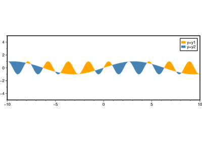
Fill the area between two horizontal curves.
This method is a high-level wrapper around
pygmt.Figure.plotto fill the area between a primary curvey(x)and a secondary curvey2(x). They2parameter can be either a single value [Default is 0] or a sequence with the same length asxandy.- Parameters:
y2 (
float|Sequence[float], default:0) – Y-coordinates of the secondary curve. It can be a scalar value for a horizontal reference line, or a sequence with the same length asxandy. Default is 0.fill (
str|None, default:None) – Fill for areas where the primary curve is greater than the secondary curve.fill2 (
str|None, default:None) – Fill for areas where the secondary curve is greater than the primary curve.pen (
str|None, default:None) – Pen attributes for the primary curve.pen2 (
str|None, default:None) – Pen attributes for the secondary curve.label (
str|None, default:None) – Label for the primary curve, to be displayed in the legend.label2 (
str|None, default:None) – Label for the secondary curve, to be displayed in the legend.projection (
str|None, default:None) – projcode[projparams/]width|scale. Select map projection.region (str or list) – xmin/xmax/ymin/ymax[+r][+uunit]. Specify the region of interest.
frame (
Frame|Axis|Literal['none'] |str|Sequence[str] |bool, default:False) – Set frame and axes attributes for the plot. It can be a bool,"none", apygmt.params.Frameorpygmt.params.Axisobject. Raw GMT strings or sequences of strings are also supported for backward compatibility. Ifframe=True, the frame will be drawn with the default attributes. Ifframe="none", no frame will be drawn. Use apygmt.params.Frameorpygmt.params.Axisobject for more control over the attributes of the frame and axes. A tutorial is available at frame and axes attributes. Full documentation is at https://docs.generic-mapping-tools.org/6.6/gmt.html#b-full.verbose (bool or str) – Select verbosity level [Full usage].
panel (
int|Sequence[int] |bool, default:False) –Select a specific subplot panel. Only allowed when used in
Figure.subplotmode.Trueto advance to the next panel in the selected order.index to specify the index of the desired panel.
(row, col) to specify the row and column of the desired panel.
The panel order is determined by the
Figure.subplotmethod. row, col and index all start at 0.perspective (
float|Sequence[float] |str|bool, default:False) –Select perspective view and set the azimuth and elevation of the viewpoint.
Accepts a single value or a sequence of two or three values: azimuth, (azimuth, elevation), or (azimuth, elevation, zlevel).
azimuth: Azimuth angle of the viewpoint in degrees [Default is 180, i.e., looking from south to north].
elevation: Elevation angle of the viewpoint above the horizon [Default is 90, i.e., looking straight down at nadir].
zlevel: Z-level at which 2-D elements (e.g., the plot frame) are drawn. Only applied when used together with
zsizeorzscale. [Default is at the bottom of the z-axis].
Alternatively, set
perspective=Trueto reuse the perspective setting from the previous plotting method, or pass a string following the full GMT syntax for finer control (e.g., adding+wor+vmodifiers to select an axis location other than the plot origin). See https://docs.generic-mapping-tools.org/6.6/gmt.html#perspective-full for details.transparency (float) – Set transparency level, in [0-100] percent range [Default is
0, i.e., opaque]. Only visible when PDF or raster format output is selected. Only the PNG format selection adds a transparency layer in the image (for further processing).
Examples
>>> import numpy as np
>>> import pygmt
>>> x = np.linspace(0, 2 * np.pi, 200)
>>> fig = pygmt.Figure()
>>> fig.fill_between(
...     x=x,
...     y=np.sin(2 * x),
...     y2=np.sin(3 * x),
...     region=[0, 4 * np.pi, -1.2, 1.2],
...     projection="X10c/4c",
...     frame=True,
...     fill="lightblue",
...     pen="1p,blue",
...     fill2="lightred",
...     pen2="1p,red",
... )
>>> fig.show()